Solution Method for Nonlinear Integral Equations

EqWorld

The World of Mathematical Equations

Home Page Exact Solutions Methods Software Education For Authors Math Forums

A Solution Method for Some Classes of Nonlinear Integral, Integro-Functional, and Integro-Differential Equations

Published in Doklady Mathematics as: A. D. Polyanin, A. I. Zhurov, Exact solutions to some classes of nonlinear integral, integro-functional, and integro-differential equations, Doklady Mathematics, 2008, Vol. 77, No. 2, pp. 315-319.

Abstract

A method for constructing exact solutions to some classes of Urysohn-type integral equations (with constant limits of integration) is suggested. It generalizes the method for solving nonlinear integral equations of the second kind with a degenerate kernel. The method is based on the solution of the auxiliary linear equation obtained by discarding the nonlinear terms. Some new solutions to specific nonlinear integral equations of the first and second kind are obtained. The generalization of the method to some nonlinear integro-functional, and integro-differential equations is discussed and illustrative examples are given.

1. Introduction

There are a considerable number of methods for finding exact solutions to various classes of linear integral equations (e.g., see [1–20]). Numerous exact solutions obtained with these methods have been collected and systematized in the handbook [20]. Unlike linear equations, only a small number of exact solutions to nonlinear integral equations are known [4, 19, 20].

2. Description of the method for nonlinear integral equations

To make it easier to understand, let us first present the method as applied to constructing exact solutions to nonlinear integral equations. After that, its generalization to more complex equations will be given.

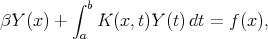
Let us consider nonlinear integral equations with constant limits of integration (Urysohn-type equations) of the form

$∫ b[ ∑n ] βy (x) + K (x, t)y (t) + φm (x)Ψm (t,y(t)) dt = f(x). a m=1$
(1)

To β = 0 there correspond equations of the first kind and to β = 1, equations of the second kind. In the special case φ₁(x) = = φ_n(x) = 0, equation (1) becomes a linear integral equation. If β = 1 and K(x,t) = 0, it is a nonlinear integral equation with a degenerate kernel. In the latter case, solutions to equation (1) are sought in the form of a finite sum, y(x) = f(x) + ∑ A_mφ_m(x), where the constants A_m are determined by solving a system of nonlinear algebraic (transcendental) equations [4, 19, 20].

Consider the auxiliary linear integral equation

$∫ b βY (x ) + K (x,t)Y (t)dt = f(x), a$
(2)

which is obtained from (1) by discarding the nonlinear terms. Suppose now that equation (2) can be solved for any function f(x) from some class of functions L_F. Let Y_f(x) denote a solution to the truncated equation (2).

Let φ_m(x) L_F (m = 1, …, n). Then the function

$n y(x ) = Y (x ) + ∑ A Y (x), f m=1 m φm$
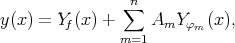(3)

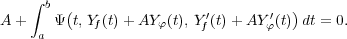
solves the original nonlinear equation (1). The function Y_{φ_m}(x) in (3) is a solution to the linear equation (2) where f(x) is substituted by φ_m(x). Inserting (3) into (1), collecting the coefficients of f(x), φ₁(x), …, φ_n(x), and equating the coefficients to zero, one arrives at the following system of nonlinear algebraic (transcendental) equations for the constants A_m:

$∫ b ( ∑n ) Am + Ψm t, Yf(t) + AjY φj(t) dt = 0, m = 1, ...,n. a j=1$
(4)

In general, formulas (3)–(4) may determine several (or infinitely many) solutions to the nonlinear integral equation (1). In the special case of a linear equation (1) with Ψ_m(t,y) = φ_m(t)y, the algebraic system (4) is linear and determines (in the nondegenerate case) a single solution.

Remark 1. The above method may be used for approximate solution of nonlinear integral equations of the more general case

∫ βy(x)+ b[K (x,t)y(t) + Ψ(x,t,y(t))]dt = f (x) a

by suitably approximating the nonlinear part of the kernel as Ψ(x,t,y(t)) ≈∑ φ_m(x)Ψ_m(t,y(t)).

Remark 2. In the special case of β = 1 and K(x,t) = 0, we have Y_f(x) = f(x). Then the above method converts into the known method for nonlinear integral equations of the second kind with constant limits of integration and a degenerate kernel [4, 19, 20].

3. Examples of exact solutions to nonlinear integral equations

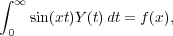
Example 1. Consider the integral equation of the first kind with a quadratic nonlinearity

$∫ ∞ [sin(xt)y(t)+ φ(x)ψ(t)y2(t)]dt = f(x ). 0$
(5)

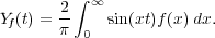
The auxiliary linear integral equation

$∫ ∞ 0 sin(xt)Y (t)dt = f(x),$
(6)

obtained from (5) by setting φ(x) = 0, is the Fourier sine transform up to a constant factor [6, 14, 20, 21]. Is solution is given by

$∫ -2 ∞ Yf(t) = π 0 sin(xt)f(x )dx.$
(7)

Solutions of the original nonlinear equation (5) are sought in the form

$2-∫ ∞ y(t) = Yf(t)+ AY φ(t), Yφ(t) = π 0 sin(xt)φ(x)dx.$
(8)

Substituting (8) into (5) and rearranging he terms, one arrives at a quadratic equation for the coefficients A:

$2 pA + qA + r = 0,$
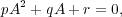(9)

where

∫ ∞ ∫ ∞ ∫ ∞ p = ψ(t)Y2φ(t)dt, q = 1 + 2 ψ(t)Yf(t)Yφ(t)dt, r = ψ(t)Yf2 (t)dt. 0 0 0

Here and henceforth, it is assumed that all integrals exist. Different solutions (8) correspond to different roots of the quadratic equation.

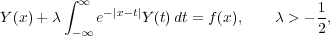
Example 2. Consider the nonlinear integral equation of the second kind

$∫ ∞ y(x)+ [λe-|x-t|y(t)+ φ(x)Ψ(t, y(t))]dt = f(x), λ > - 1. -∞ 2$
(10)

The solution to the auxiliary linear integral equation of the second kind

$∫ ∞ -|x-t| 1 Y (x )+ λ -∞ e Y(t)dt = f(x), λ > - 2,$
(11)

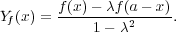
is expressed as [7, 20]

$λ ∫ ∞ ( √ ------ ) Yf(x) = f(x)- √1+-2λ- exp - 1+ 2λ |x - t| f(t)dt. -∞$
(12)

Solutions of the original nonlinear equation (10) is sought in the form

$y(x) = Yf(x)+ AY φ(x),$
(13)

where Y_φ(x) is defined by (12) with f(x) substituted by φ(x). On inserting (13) into (10), one arrives at the following algebraic (transcendental) equation for the coefficient A:

$∫ b A + Ψ(t, Yf(t)+ AY φ(t))dt = 0. a$
(14)

In the special case Ψ(t,y) = ψ(t)y, equation (10) is linear and its solution is given by (13) with

∫ ∞ ---0-ψ-(t)Yf(t)-dt-- A = - ∫ ∞ . 1+ 0 ψ(t)Yφ(t)dt

In the case of quadratic nonlinearity, Ψ(t,y) = ψ(t)y², equation (14) is reduced to the quadratic equation (9) where the functions Y_f(x) and Y_φ(x) are the same as above.

4. Generalizations

The method described above for Urysohn-type integral equations of the first and second kind admits a significant generalization.

Consider the abstract nonlinear equation for y = y(x)

$∑n L [y ] + φm (x)Im[y] = f(x), m=1$
(15)

where L[y] is a linear operator (integral, functional, differential,¹ or any other) and the I_m[y] are some nonlinear functionals (i.e., numbers for each y(x) from a given class of functions).

Examples of nonlinear functionals:

( ) ∫ b ( ) I1[y] = ay2(0)+ by(1), I2[y] = 0m≤axx≤1 a|y(x)|+ b|y′x(x)| , I3[y] = K t,y(t),y′t(t),y′t′t(t) dt. a

Suppose the truncated linear equation

$L[Y ] = f (x),$
(16)

obtained from (15) by discarding the nonlinear terms (i.e., setting φ_m(x) = 0, m = 1,…,n), can be solved for any f(x) from a given class of functions L_F. Let Y_f(x) denote the solution to the truncated equation (16).

Let φ_m(x) L_F (m = 1, …, n). Then the original nonlinear equation (15) has solutions of the form

$∑n y(x ) = Yf (x ) + AmY φm(x), m=1$
(17)

where Y_{φ_m}(x) is the solution to the linear equation (16) where f(x) is substituted by φ_m(x). Inserting (17) into (15), collecting the coefficients of the functions f(x), φ₁(x), …, φ_n(x), and equating the coefficients to zero, one arrives at the following system of nonlinear algebraic (transcendental) equations for A_m:

$[ ∑n ] Am + Im Yf(x) + AjY φj(x) , m = 1,...,n. j=1$
(18)

Formulas (17)–(18) can determine several (or even infinitely many) solutions to equation (15).

5. Examples of exact solutions to nonlinear integro-functional and integro-differential equations

Example 3. Consider the nonlinear functional-integral equation

$∫ a ( ) y(x)+ λy(a - x )+ φ(x) 0 Ψ t,y(t),y(a- t) dt = f(x), λ ⁄= ±1,$
(19)

where 0 ≤ x ≤ a and 0 ≤ t ≤ a.

The auxiliary linear functional equation, obtained from (19) by setting φ(x) = 0, is expressed as

$Y (x) +λY (a- x) = f(x ).$
(20)

Let us substitute x in (20) by a − x to obtain

$Y (a- x)+ λY (x) = f(a- x).$
(21)

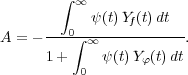
Eliminating Y (a - x) from (20)–(21), one finds the solution to functional equation (20):

$f(x)--λf(a--x)- Yf(x ) = 1- λ2 .$
(22)

Following the method described in Section 4, one looks for solutions to the original functional-integral equation (19) in the form

φ-(x)-- λ-φ(a--x) y(x) = Yf(x)+ AY φ(x), Yφ(x) = 1- λ2 ,

where the constant A is determined by the algebraic (transcendental) equation

∫ a A + Ψ(t, Y (t)+ AY (t), Y (a- t)+ AY (a - t))dt = 0. 0 f φ f φ

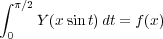
Example 4. Consider the nonlinear integral-functional-differential equation

$∫ π∕2[ ( ′ )] 0 y(x sint)+ φ(x)Ψ t, y(t), yt(t) dt = f (x).$
(23)

Note that this equation involves the unknown function with two different arguments, y(xsint) and y(t).

The auxiliary linear equation, obtained from (23) by setting φ(x) = 0, has the form

∫ π∕2 Y (xsin t)dt = f(x ) 0

and is called Schlömilch’s equation. Its solution is expressed as [11]

[ ∫ π∕2 ] Yf(z) = 2 f(0)+ z f′ξ(ξ)dτ , ξ = zsinτ. π 0

Following the method described in Section 4, one looks for solutions to the original integral-functional-differential equation (23) in the form

y(z) = Yf(z)+ AYφ(z), 2 [ ∫ π∕2 ] Yφ(z) =-- φ(0)+ z φ′ξ(ξ)dτ , ξ = zsinτ. π 0

The constant A is determined by the algebraic (transcendental) equation

∫ b ( ) A + Ψ t, Yf(t) +AY φ(t), Yf′(t)+ AY ′φ(t) dt = 0. a

Example 5. Consider the boundary-value problem for the nonlinear integro-differential equation

$∫ y′′ + φ(x) 1Ψ (t,y(t))dt = f(x) xx 0$
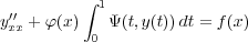(24)

with the homogeneous boundary conditions

$y(0) = y(1) = 0.$
(25)

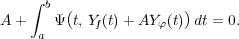
The solution of the auxiliary linear boundary-value problem

Yx′′x = f (x); Y(0) = Y (1) = 0

is expressed as

$∫ 1 { Yf(x) = G (x,ξ)f(ξ)dξ, G(x,ξ) = (ξ - 1)x for 0 ≤ x ≤ ξ ≤ 1, 0 (x- 1)ξ for 0 ≤ ξ ≤ x ≤ 1.$
(26)

Therefore solutions to the original boundary-value problem for the nonlinear integro-differential equation (24) subject to the boundary conditions (25) are sought in the form

$y(x) = Yf(x)+ AY φ(x).$
(27)

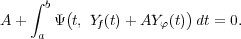
The function Y_φ(x) is determined by the right-hand side of the first formula in (26), where f(x) is substituted by φ(x). Inserting (27) into (24), one arrives at the following algebraic (transcendental) equation for the coefficient A:

$∫ b ( ) A + a Ψ t, Yf(t)+ AY φ(t) dt = 0.$
(28)

In the special case of f(x) = 0 and φ(x) = 1, one should set Y_f(x) = 0 and Y_φ(x) = x(x - 1) in (27)–(28).

Remark 3. In the case of nonhomogeneous boundary conditions for integro-differential equations, one should perform the change of variable y(x) = (x) + g(x), where g(x) is any sufficiently smooth function satisfying the boundary conditions, to obtain a problem for (x) with homogeneous boundary conditions. For example, if the integro-differential equation (24) is subjected to the nonhomogeneous boundary conditions y(0) = a and y(1) = b, one could take g(x) = a + (b - a)x.

References

Lovitt, W. V., Linear Integral Equations, Dover Publ., New York, 1950.
Petrovskii, I. G., Lectures on the Theory of Integral Equations, Graylock Press, Rochester, 1957.
Mikhlin, S. G., Linear Integral Equations, Hindustan Publ. Corp., Delhi, 1960.
Krasnov, M. L., Kiselev, A. I., and Makarenko, G. I., Problems and Exercises in Integral Equations, Mir Publ., Moscow, 1971.
Cochran, J. A., The Analysis of Linear Integral Equations, McGraw-Hill Book Co., New York, 1972.
Zabreyko, P. P., Koshelev, A. I., et al., Integral Equations: A Reference Text, Noordhoff Int. Publ., Leyden, 1975.
Gakhov, F. D. and Cherskii, Yu. I., Equations of Convolution Type [in Russian], Nauka, Moscow, 1978.
Tricomi, F. G., Integral Equations, Dover Publ., New York, 1985.
Jerry, A. J., Introduction to Integral Equations With Applications, Marcel Dekker, New York–Basel, 1985.
Gorenflo, R. and Vessella, S., Abel Integral Equations: Analysis and Applications, Springer-Verlag, Berlin–New York, 1991.
Corduneanu, C., Integral Equations and Applications, Cambridge Univ. Press, Cambridge, 1991.
Pipkin, A. C., A Course on Integral Equations, Springer-Verlag, New York, 1991.
Kondo, J., Integral Equations, Clarendon Press, Oxford, 1991.
Prudnikov, A. P., Brychkov, Yu. A., and Marichev, O. I., Integrals and Series, Vol. 5, Inverse Laplace Transforms, Gordon & Breach, New York, 1992.
Samko, S. G., Kilbas, A. A., and Marichev, O. I., Fractional Integrals and Derivatives. Theory and Applications, Gordon & Breach Sci. Publ., New York, 1993.
Hackbusch, W., Integral Equations: Theory and Numerical Treatment, Birkhäuser Verlag, Boston, 1995.
Sakhnovich, L. A., Integral Equations with Difference Kernels on Finite Intervals, Birkhäuser Verlag, Basel–Boston, 1996.
Kanwal, R. P., Linear Integral Equations, Birkhäuser Verlag, Boston, 1996.
Verlan’, A. F. and Sizikov V. S., Integral Equations: Methods, Algorithms, and Programs [in Russian], Naukova Dumka, Kiev, 1986.
Polyanin, A. D. and Manzhirov, A. V., Handbook of Integral Equations, CRC Press, Boca Raton, 1998.
Ditkin, V. A. and Prudnikov, A. P., Integral Transforms and Operational Calculus, Pergamon Press, New York, 1965.

A.D. Polyanin and A.I. Zhurov, A solution method for some classes of nonlinear integral, integro-functional, and integro-differential equations, 2007. Website EqWorld — The World of Mathematical Equations, http://eqworld.ipmnet.ru/en/methods/ie/ie-meth3.htm