N.A. Kudryashov. Seven common errors in finding exact solutions of nonlinear differential equations - 2. First error...

EqWorld

The World of Mathematical Equations

Exact Solutions Methods Software For Authors Math Forums

Exact Solutions > Interesting Papers > N.A. Kudryashov. Seven common errors in finding exact solutions of nonlinear differential equations > 2. First error...

Seven common errors in finding exact solutions of nonlinear differential equations
© N.A. Kudryashov
Communications in Nonlinear Science and Numerical Simulation (to be pubslished in 2009)

2. First error: some authors use equivalent methods to find exact solutions

In this section we start to discuss common errors to search for the exact solutions of nonlinear differential equations. We observed these errors by studying many papers in the last years.

Many authors try to introduce ”new methods” to look for ”new solutions” of nonlinear differential equations and many investigators hope that using different approaches they can find new solutions. However analyzing numerous applications of many methods we discover that many of them are equivalent each other and in many cases it is impossible to obtain something new.

So the first error can be formulated as follows.

First error. Some authors use the equivalent methods to find the exact solutions of nonlinear differential equations, but believe that they can find new exact solutions.

Using the solitary wave solutions of the KdV - Burgers equation let us show that many methods to look for the exact solutions of nonlinear differential equations are equivalent.

Example 1a. Application of the truncated expansion method.

The truncated expansion method was introduced in [9, 10] and developed in many papers to obtain the Lax pairs, the Backlund transformations and the rational solutions for the integrable equations [11]. This approach was also used in the papers [12, 13, 14, 15, 16, 17, 18, 19, 20, 21] to search for the exact solutions of nonintegrable differential equations.

Consider the application of the truncated expansion method in finding the exact solutions of the KdV - Burgers equation
$ut + u ux + β uxxx = μ uxx.$ (2.1)

Substituting u(x,t) in the form [9]
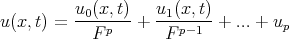$u (x,t) u (x,t) u (x,t) = -0-----+ -1------+ ...+ up F p F p-1$ (2.2)

into the KdV - Burgers equation Eq.(2.1) and finding the order of the pole p = 2 for the solution u(x,t) and functions u0(x,t) and u1(x,t) we obtain the transformation [12]
$∂2 ln F 12μ ∂ ln F u(x,t) = 12β ----2--- ---- ------+ u2. ∂x 5 ∂x$ (2.3)

Assuming [12]
$F = 1 + C1 exp (kx - ωt) u2 = C2,$ (2.4)

(where C₁ and C₂ are arbitrary constants), we have the system of algebraic equations with respect to k and . Solving this algebraic system we have the values of k and as follows
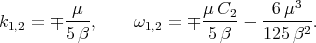$-μ- μ-C2- -6μ3--- k1,2 = ∓ 5β , ω1,2 = ∓ 5β - 125β2 .$ (2.5)

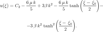
For these values of k and the solitary wave solutions for the KdV - Burgers equation takes the form [12]
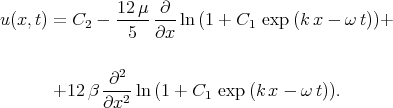$12μ- ∂-- u(x,t) = C2 - 5 ∂x ln (1 + C1 exp (kx - ω t))+ 2 +12 β -∂--ln(1 + C exp (k x - ω t)). ∂x2 1$ (2.6)

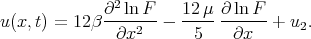
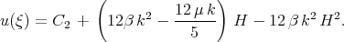
We can see that solution (2.6) satisfies the nonlinear ordinary differential equation in the form
$β k3U ξξξ - μ k2U ξξ + k U U ξ - ω U ξ = 0, ξ = k x - ω t.$ (2.7)

We have found exact solution of the KdV — Burgers equation in essence using the travelling wave solutions although we tried to look for more general solutions. Many researches look for the exact solutions taking directly into account the travelling wave solutions.

Example 1b. Application of the Riccati equation as the simplest equation (the first variant) [22, 23, 24, 25, 26].

Solution (2.6) can be written as
$C1-(60β-k2 --12μ-k)-exp-(ξ-) 12β-C21-k2-exp(2-ξ)- u(ξ) = C2 + 5(1 + C1 exp (ξ)) - (1 + C1 exp(ξ))2 .$ (2.8)

Consider the expression
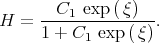$--C1-exp-(ξ)--- H = 1 + C exp (ξ). 1$ (2.9)

Taking the derivative of the function H with respect to we get
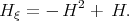$2 Hξ = - H + H.$ (2.10)

We obtain that solution (2.8) can be written in the form
$( ) 2 12-μk- 2 2 u(ξ) = C2 + 12β k - 5 H - 12 β k H .$ (2.11)

Eq.(2.11) means that one can look for the solution of the KdV - Burgers equation using the expression
$u(ξ) = A0 + A1 H + A2 H2,$ (2.12)

where H is the solution of Eq.(2.10). It is seen, that the application of the simplest equation method with the Riccati equation gives the same results as the truncated expansion method.

Example 1c. Application of the tanh - function method [27, 28, 29, 30].

Expression (2.9) can be transformed as follows
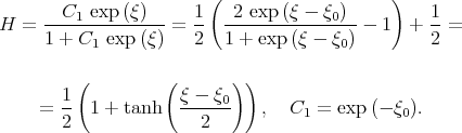$( ) H = --C1-exp-(ξ)-- = 1- -2-exp-(ξ --ξ0)-- 1 + 1-= 1 + C1 exp (ξ) 2 1 + exp (ξ - ξ0) 2 ( ( )) 1- ξ---ξ0 = 2 1 + tanh 2 , C1 = exp (- ξ0).$ (2.13)

From (2.13) we have that solution (2.8) of the KdV - Burgers equation can be written in the form
$( ) u(ξ) = C2 - 6μ-k-+ 3β k2 - 6-μk-tanh ξ --ξ0- - 5 5 2 ( ) 2 2 ξ----ξ0- - 3β k tanh 2 .$ (2.14)

Substituting k1,2 and ω1,2 into solution (2.14) we have the solution of the KdV - Burgers equation in the form [12]
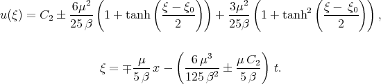$( ( )) ( ( ) ) 6μ2 ξ - ξ0 3μ2 2 ξ - ξ0 u (ξ) = C2 ± ----- 1 + tanh ------ + ---- 1 + tanh ------- , 25 β 2 25β 2 μ ( 6μ3 μ C ) ξ = ∓ --- x - -----2-± ---2- t. 5 β 125β 5β$ (2.15)

We obtain that the solution of the KdV - Burgers equation can be found as the sum of the hyperbolic tangents
$u(ξ) = A0 + A1 tanh [m (ξ - ξ0)] + A2 tanh2 [m (ξ - ξ0)],$ (2.16)

where m is unknown parameter.

We have obtained that the tanh - function method is equivalent in essence to the truncated expansion method. As this fact takes place we can see that the maximum power of the hyperbolic tangent in (2.16) coincides with the order of the pole for the solution of the KdV - Burgers equation.

Example 1d. Application of the Riccati equation as the simplest equation (the second variant). [22, 23, 24].

Note that the function
$Y(ξ) = m tanh [m (ξ - ξ0)]$ (2.17)

is the general solution of the Riccati equation
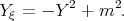$Yξ = - Y 2 + m2.$ (2.18)

From (2.16) we obtain, that we can look for the solution of the KdV - Burgers equation taking into account the formula
$2 u(ξ) = A0 + A1 Y + A2 Y ,$ (2.19)

where Y satisfies Eq.(2.18). The maximum power of the function Y in (2.19) coincides with the pole of the solution for the KdV - Burgers equation.

Example 1e. Application of the $G ξ∕G$ method [31, 32, 33].

Taking into account the transformation
$Y = Gξ- G$ (2.20)

we reduce Eq.(2.18) to the linear equation
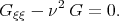$2 G ξξ - ν G = 0.$ (2.21)

As this fact takes place expression (2.19) can be written in the form
$( )2 u(ξ) = A + A G-ξ + A G-ξ . 0 1 G 2 G$ (2.22)

This means, that we can search for the exact solutions of the KdV - Burgers equation in the form (2.22), where G (ξ) satisfies Eq.(2.21). We obtain, that application of the G ξ∕G method is equivalent to application of the simplest equation method with the Riccati equation, to the tanh - function method and to the truncated expansion method.

Note that the G ξ∕G method follows directly from the truncated expansion method because solution (2.3) can be written as
$2 u(x,t) = u - 12-μ Fx-- 12β F-x + 12β Fxx-. 2 5 F F 2 F$ (2.23)

Assuming that the function F (x,t) satisfies linear equation of the second order
$Fxx = m0 Fx + m1 F + m2,$ (2.24)

where m₀, m₁ and m₂ are unknown parameters we have the expression (2.22) for Fξ∕F . So, the G ξ∕G - method coincides with the truncated expansion method if we use the travelling wave solutions.

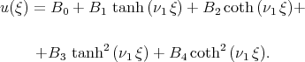
Example 1f. Application of the tanh — coth method [34, 35, 36].

Assuming in (2.16) iπ ξ0 = -2 , we obtain the formula
$u(ξ) = A0 + A1 coth(ν ξ) + A2 coth2(ν ξ).$ (2.25)

This means that we can search for the solution of the KdV - Burgers equation in the form (2.25).

Using the identity for the hyperbolic functions in the form
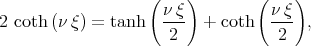$( ) ( ) ν ξ ν ξ 2 coth(ν ξ) = tanh --- + coth --- , 2 2$ (2.26)

and substituting (2.26) into (2.25) we have the tanh - coth method to look for the solitary wave solutions of the KdV - Burgers equation
$u(ξ) = B0 + B1 tanh (ν1ξ) + B2 coth(ν1 ξ)+ +B tanh2 (ν ξ) + B coth2 (ν ξ). 3 1 4 1$ (2.27)

We have obtained, that the tanh - coth method is equivalent to the truncated expansion method too and we cannot find new exact solutions of the KdV - Burgers equation by the tanh - coth method.

Example 1g. Application of the Exp - function method [37, 38, 39, 40, 41].

Solution (2.8) of the KdV - Burgers equation can be written in the form
$5C2e--ξ +-C1(60βk2----12μk-+-10C2-) +-5C21(C2---12-βk2)eξ u(ξ) = 5 e-ξ + 10 C1 + 5 C21 eξ .$ (2.28)

This solution can be found if we look for a solution of the KdV — Burgers equation using the Exp - function method in the form
$a e-ξ + a + a eξ u(ξ) = -0---ξ----1----2-ξ . b0 e + b1 + b2e$ (2.29)

Using the Exp - function method to search for the exact solutions of the KdV - Burgers equation one can have again the solitary wave solutions (2.3) with the functions (2.4) and the parameters (2.5). Studying the application of the Exp - function method we obtain that this method provides no new exact solutions of nonlinear differential equations in comparison with other methods. Moreover the Exp - function method do not allow us to find the order of the pole for the solution of nonlinear differential equation [42]. Usually the authors use a few variants of fractions with the sum of exponential functions to look for the solitary wave solutions.

The EqWorld website presents extensive information on solutions to various classes of ordinary differential equations, partial differential equations, integral equations, functional equations, and other mathematical equations.

Seven common errors in finding exact solutions of nonlinear differential equations © N.A. Kudryashov Communications in Nonlinear Science and Numerical Simulation (to be pubslished in 2009)

Contents

2. First error: some authors use equivalent methods to find exact solutions

Seven common errors in finding exact solutions of nonlinear differential equations
© N.A. Kudryashov
Communications in Nonlinear Science and Numerical Simulation (to be pubslished in 2009)