|
|
EqWorld The World of Mathematical Equations |
 |
Exact Solutions > Interesting Papers > N.A. Kudryashov. Seven common errors in finding exact solutions of nonlinear differential equations > 5. Fourth error...
Seven common errors in finding exact solutions of nonlinear differential equations
© N.A. Kudryashov
Communications in Nonlinear Science and Numerical Simulation (to be pubslished in 2009)
Contents
- Abstract
- Introduction
- First error: some authors use equivalent methods to find exact solutions
- Second error: some authors do not use the known general solutions of ordinary differential equations
- Third error: some authors omit arbitrary constants after integration of equation
- Fourth error: using some functions in finding exact solutions some authors lose arbitrary constants
- Fifth error: some authors do not simplify the solutions of differential equations
- Sixth error: some authors do not check solutions of differential equations
- Seventh error: some authors include additional arbitrary constants into solutions
- Conclusion
- References
5. Fourth error: using some functions in finding exact solutions some authors lose arbitrary constants
Some authors do not include the arbitrary constants in finding the exact solutions of nonlinear differential equations. As a result these authors obtain many solutions, that can be determined as the only solution using some arbitrary constants. The arbitrary constants can be included, if we use the general solutions of the known differential equations. Sometimes this error can be corrected, using the property of the autonomous differential equation. So, the fourth error can be formulated as follows.
Fourth error. Using some functions in finding the exact solutions of nonlinear differential equations some authors lose the arbitrary constants.
Let us explain this error. Consider an ordinary differential equation in the general form
 | (5.1) |
Let us assume that Eq. (5.1) is autonomous and this equation admits the shift of the independent variable  (where C2 is an arbitrary constant). This means that the constant C2 added to the variable
  in Eq.(5.1) does not change the form of this equation. In this case Eq.(5.1) is invariant under the shift of the independent variable.
Taking this property into account, we obtain the advantage for the solution of Eq. (5.1). If we know a solution  of Eq. (5.1), then for the autonomous equation we have a solution
  of this equation with additional arbitrary constant
  .
.
The main feature of the autonomous equation is that the fact that the solution  is more general, then
  .
.
The error discussed often leads to a huge amount of different expressions for the solutions of nonlinear differential equations instead of choosing one solution with an arbitrary constant  .
.
The application of the tanh - function method [28, 29, 30] for finding the exact solutions allows us to have the special solutions of nonlinear differential equations as a sum of hyperbolic tangents  . However for the autonomous equation such types of the solutions can be taken as the more general solution in the form
  .
.
Example 4a. Solution of the Riccati equation
 | (5.2) |
Eq. (5.2) is of the first order, therefore the general solution of Eq. (5.2) depends on the only arbitrary constant. We can meet a lot of ”different” solutions of Eq. (5.2). For example
 | (5.3) |
 | (5.4) |
 | (5.5) |
 | (5.6) |
In fact, the general solution of Eq. (5.2) takes the form
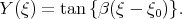 | (5.7) |
All solutions (5.3) - (5.6) can be obtained from the general solution (5.7) of the Riccati equation, because of the following equalities
 | (5.8) |
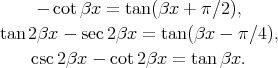
Example 4b. Solution of the Cahn - Hilliard equation by Ugurlu and Kaya [57]
 | (5.9) |
Eq.(5.9) was considered in [57] by means of the modified extended tanh - function method by Ugurlu and Kaya. Using the travelling wave
 | (5.10) |
the authors obtained the exact solutions of the equation
 | (5.11) |
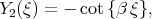
They found eight solutions of Eq.(5.11) at c = 1. Six solutions are the following
 | (5.12) |
 | (5.13) |
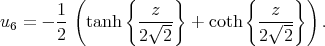 | (5.14) |
However all these solutions can be written as the only solution with an arbitrary constant z0
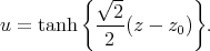 | (5.15) |
Note, that Eq.(5.11) at c = 1 takes the form
 | (5.16) |
Twice integrating Eq.(5.16) with respect to z, we have
 | (5.17) |
where C1 and C2 are arbitrary constants. At C1 = 0 the solution of Eq.(5.17) is expressed via the Jacobi elliptic function.
Example 4c. Solution of the KdV - Burgers equation by Soliman [51]
 | (5.18) |
Using the travelling wave and ”the modified extended tanh - function method” the author [51] obtained four solutions of Eq.(5.18). Three of them take the form
![2 [ ( ) ( ) ] 2 -ν--- -νξ- 2 -νξ- 6ν-t- u(x,t) = 25ɛμ 9 - 6 coth 10μ - 3 coth 10μ , ξ = x - 25μ ;](k7e198x.png) | (5.19) |
![[ ( ) ( ) ] -ν2-- -νξ- 2 -νξ- 6ν2t- u (x,t) = 25ɛμ 9 - 6 tanh 10μ - 3 tanh 10 μ , ξ = x - 25μ ;](k7e199x.png) | (5.20) |
![2 [ ( ( ) ( )) u (x,t) = 3-ν-- 1 - -4- tanh -νξ- + coth ν-ξ- - 25ɛμ 10 20μ 20μ ( ( ) ( ) )] 1-- 2 ν-ξ- 2 -νξ- 6ν2t- - 10 tanh 20μ + coth 20 μ , ξ = x - 25μ .](k7e200x.png) | (5.21) |
All these solutions can be written in the form
![[ ( ) ( ) ] 3 ν2 νξ 2 ν ξ u(x,t) = ----- 3 - 2 tanh ---- - ξ0 - tanh ----- ξ0 , 25ɛμ 10μ 10μ 6ν2t ξ = x - ----. 25μ](k7e201x.png) | (5.22) |
Assuming  in (5.22), we obtain solution (5.20). In the case
  in (5.22) we have solution (5.19). Taking into account the formulae
 | (5.23) |
 | (5.24) |
we can transform solution (5.22) into solution (5.21).
We can see, that these solutions do not differ, if we take the constant  into account in one of these solutions.
The fourth solution by Soliman [51] can be simplified as well. All the solutions by the KdV — Burgers equation by Soliman coincides with (2.15).
Example 4d. Solution of the combined KdV - mKdV equation by Bekir [58]
 | (5.25) |
Using the extended tanh method the author [58] have obtained the following solutions of Eq.(5.25)
![12r u = ----[1 + tanh (x - 4rt)], p](k7e208x.png) | (5.26) |
![12r u = ----[1 + coth(x - 4rt)], p](k7e209x.png) | (5.27) |
![24r u = ----[(21 + tanh (x - 4rt)) + (1 + coth (x - 4rt))]. p](k7e210x.png) | (5.28) |
All these solutions can be written as the only solution with an arbitrary constant
![u = 12r[1 + tanh (x - 4rt + φ )]. p 0](k7e211x.png) | (5.29) |
Example 4e. Solution of the coupled Hirota — Satsuma — KdV equation by Bekir [59]
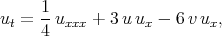 | (5.30) |
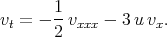 | (5.31) |
The system of Eqs.(5.30) and (5.31) was studied by means of the tanh - coth method by Bekir [59]. Using the travelling wave 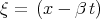 the author obtained the system of equations
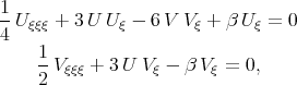 | (5.32) |
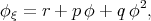
and gave ten solitary wave solutions. However all the solitary wave solutions of the system of equations (5.30) and (5.31) by Bekir [59] can be expressed by the formulae
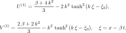 | (5.33) |
(where k,  and
and  are arbitrary constants)
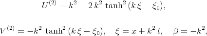 | (5.34) |
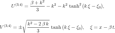 | (5.35) |
Example 4f. ”Twenty seven solution” of the ”generalized Riccati equation” by Xie, Zhang and Lü [60].
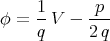
The authors [60] ”firstly extend” the Riccati equation to the ”general form”
 | (5.36) |
where r, p and q are the parameters. They ”fortunately find twenty seven solutions” of Eq.(5.36).
It was very surprised that the authors are not aware that the solution of Eq.(5.36) was known more then one century ago. It is very strange but these 27 solutions was repeated by Zhang [61] as the important advantage.
Let us present the general solution of Eq.(5.36). Substituting
 | (5.37) |
into Eq.(5.36) we have
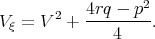 | (5.38) |
Assuming
 | (5.39) |
in Eq.(5.38) we obtain the linear equation of the second order
 | (5.40) |
The general solution of Eq.(5.40) is well known
 | (5.41) |
Using formula (5.39) and (5.37) we obtain the solution of Eq.(5.36) in the form
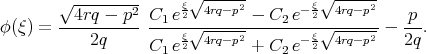 | (5.42) |
The general solution of Eq.(5.36) is found from (5.42). All 27 solutions by Xie, Zhang and Lü are found from solution (5.42) and we cannot obtain other solutions.
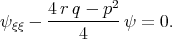
Example 4g. ”New solutions and kinks solutions” of the Sharma — Tasso — Olver equation by Wazwaz [62].
Using the extended tanh method Wazwaz [62] have found 18 solitary wave and kink solutons of the Sharma — Tasso —- Olver equation
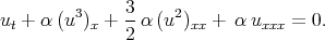 | (5.43) |
Taking the travelling wave solution 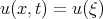 ,
,  into account the author considered the nonlinear ordinary differential equation in the form
 | (5.44) |
However Eq.(5.44) can be transformed to the second - order linear differential equation (see, example 2f)
 | (5.45) |
by the transformation
 | (5.46) |
The solution of Eq.(5.44) is given by formula (3.40) at  . Certainly all ”new solutions” of the Sharma — Tasso — Olver equation by Wazwaz [62] are found from (3.40) at
  .
.
We can see, that there is no need to write a list of all possible expressions for the solutions at the given  . It is enough to present the solution of the equation with an arbitrary constant. Moreover, the solution with arbitrary constants looks better.
The simple and powerful tool to remove this error is to plot the graphs of the expressions obtained. The expressions having the same graphs usually are equivalent.
The EqWorld website presents extensive information on solutions to various classes of ordinary differential equations, partial differential equations, integral equations, functional equations, and other mathematical equations.
Copyright © 2004-2017 Andrei D. Polyanin