|
|
EqWorld The World of Mathematical Equations |
 |
Exact Solutions > Interesting Papers > N.A. Kudryashov. Seven common errors in finding exact solutions of nonlinear differential equations > 4. Third error...
Seven common errors in finding exact solutions of nonlinear differential equations
© N.A. Kudryashov
Communications in Nonlinear Science and Numerical Simulation (to be pubslished in 2009)
Contents
- Abstract
- Introduction
- First error: some authors use equivalent methods to find exact solutions
- Second error: some authors do not use the known general solutions of ordinary differential equations
- Third error: some authors omit arbitrary constants after integration of equation
- Fourth error: using some functions in finding exact solutions some authors lose arbitrary constants
- Fifth error: some authors do not simplify the solutions of differential equations
- Sixth error: some authors do not check solutions of differential equations
- Seventh error: some authors include additional arbitrary constants into solutions
- Conclusion
- References
4. Third error: some authors omit arbitrary constants after integration of equation
Reductions of nonlinear evolution equations to nonlinear ordinary differential equations can be often integrated. However, some authors assume, that the arbitrary constants of integration are equal to zero. This error potentially leads to the loss of the arbitrary constants in the final expression. So the solution obtained in such way is less general than it could be. The third common error can be formulated as follows.
Third error. Some authors omit the arbitrary constants after integrating of the nonlinear ordinary differential equations.
Example 3a. Reduction of the Burgers equation by Soliman [51].
Soliman [51] considered the Burgers equation
 | (4.1) |
to solve this equation by so called ”the modified extended tanh - function method”.
It is well known, that by using the Cole-Hopf transformation [52, 53]
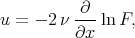 | (4.2) |
we can write the equality
 | (4.3) |
From the last relation we can see, that each solution of the heat equation
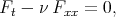 | (4.4) |
gives the solution of the Burgers equation by formula (4.2).
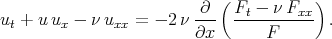
However to find the solutions of the Burgers equation Soliman [51] used the travelling wave solutions 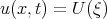 ,
,  and from Eq.(4.1) after integration with respect to
  the author obtained the equation in the form
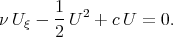 | (4.5) |
The constant of integration he took to be equal to zero. The general solution of Eq.(4.5) takes the form
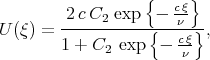 | (4.6) |
where C2 is an arbitrary constant.
The general solution of Eq.(4.5) has the only arbitrary constant. But if we take nonzero constant of integration in Eq.(4.5), we can have two arbitrary constants in the solution.
Example 3b. Reduction of the (2+1) - dimensional Konopelchenko - Dubrovsky equation by Abdou [54]
 | (4.7) |
 | (4.8) |
 he obtained the second order differential equation
 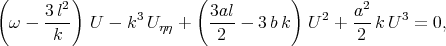 | (4.9) |
However multiplying Eq.(4.9) on  and integrating this equation with respect to
  again, we have the equation
 | (4.10) |
Example 3c. Reduction of the Ito equation by Wazwaz [55]
 | (4.11) |
The author [55] looked for the solutions of Eq. (4.11) taking into account the travelling wave
 | (4.12) |
Substituting (4.12) into (4.11) Wazwaz obtained when  and
and  the equation in the form
 | (4.13) |
Integrating Eq.(4.13) twice with respect to  one can have the equation
 | (4.14) |
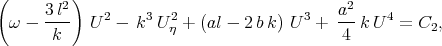
 in Eq. (4.14) we get the equation
  | (4.15) |
The general solution of this equation was discussed above in example 2b.
However the author [55] looked for solutions of Eq. (4.14) for C8 = 0 and C9 = 0 taking into consideration the tanh - coth method and did not present the general solution of Eq. (4.13).
Example 3d. Reduction of the Boussinesq equation by Bekir [32]
 | (4.16) |
 the author [32] got the equation
 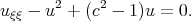 | (4.17) |
 - method, but he have been omitted two arbitrary constants after the integration.
 In fact, from Eq.(4.16) we obtain the second order differential equation in the form
 | (4.18) |
 via the first Painlevé transcendents. In the case
  solutions of Eq.(4.18) is determined by the Weierstrass elliptic function. All possible solutions of Eq. (4.16) were obtained in work [56].
The EqWorld website presents extensive information on solutions to various classes of ordinary differential equations, partial differential equations, integral equations, functional equations, and other mathematical equations.
Copyright © 2004-2017 Andrei D. Polyanin