N.A. Kudryashov. Seven common errors in finding exact solutions of nonlinear differential equations - 3. Second error...

EqWorld

The World of Mathematical Equations

Exact Solutions Methods Software For Authors Math Forums

Exact Solutions > Interesting Papers > N.A. Kudryashov. Seven common errors in finding exact solutions of nonlinear differential equations > 3. Second error...

Seven common errors in finding exact solutions of nonlinear differential equations
© N.A. Kudryashov
Communications in Nonlinear Science and Numerical Simulation (to be pubslished in 2009)

Abstract
Introduction
First error: some authors use equivalent methods to find exact solutions
Second error: some authors do not use the known general solutions of ordinary differential equations
Third error: some authors omit arbitrary constants after integration of equation
Fourth error: using some functions in finding exact solutions some authors lose arbitrary constants
Fifth error: some authors do not simplify the solutions of differential equations
Sixth error: some authors do not check solutions of differential equations
Seventh error: some authors include additional arbitrary constants into solutions
Conclusion
References

3. Second error: some authors do not use the known general solutions of ordinary differential equations

Many authors look for the solutions of nonlinear evolution equations using the travelling waves. As this fact takes place, these authors obtain nonlinear ordinary differential equations and search for the solutions of these equations. However nonlinear ordinary differential equations had been studied very well and the solutions of them were obtained many years ago. However some of the authors do not use the well - known general solutions of the ordinary differential equations. As a result these authors obtain the solutions that have already been found by other scientists.

The second error can be formulated as follows.

Second error. Some authors search for solutions of nonlinear differential equations, but do not use the known general solutions of these equations.

Example 2a. Reduction of the (2+1) - dimensional Burgers equation by Li and Zhang [43]
$ut = uuy + α v ux + β uyy + α β uxx, ux = vy.$ (3.1)

The authors [43] considered the wave transformations in the form
$u(x,y, t) = U (ξ), v(x,y, t) = V (ξ), ξ = k (x + ly + λ t),$ (3.2)

and obtained the system of the ordinary differential equations
$β k(α + l2)U ξξ + α V U ξ + lU U ξ - λU ξ = 0,$ (3.3)

$U ξ - lV ξ = 0.$ (3.4)

Li and Zhang [43] proposed ”a generalized multiple Riccati equation rational expansion method” to construct ”a series of exact complex solutions” for the system of equations (3.3) and (3.4). The authors [43] found ”new complex solutions” of the (2+1) - dimensional Burgers equation and ”brought out rich complex solutions”.

However, integrating Eq.(3.4) with respect to we have
$U = lV + C1,$ (3.5)

where C₁ is an arbitrary constant. Substituting U into Eq.(3.3) we obtain
$β k (α + l2) Vξξ + (α + l2)V Vξ + (C1 l - λ)V ξ = 0.$ (3.6)

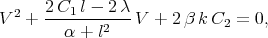
Integrating Eq.(3.6) with respect to we get the Riccati equation in the form
$( ) 1 2 2 C1 l - 2 λ V ξ = - ----- V + --------2-- V + 2 β kC2 . 2β k α + l$ (3.7)

Eq.(3.7) can be reduced to the form
$dV- -1--- dξ = - 2β k (V - V1)(V - V2),$ (3.8)

where and V 2 are the roots of the algebraic equation
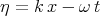
$2 2C1-l --2λ- V + α + l2 V + 2 β kC2 = 0,$ (3.9)

that take the form
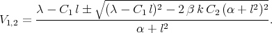$∘ ----------2----------------2-2 λ---C1-l ±--(λ---C1-l)---2-β-kC2-(α-+-l-)- V1,2 = α + l2 .$ (3.10)

Integrating Eq.(3.8) with respect to , we find the general solution of Eq.(3.7) in the form
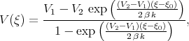$( ) V1 - V2 exp (V2-V12)β(ξk-ξ0) V (ξ ) = ---------(-(V2-V1)(ξ-ξ0))--, 1 - exp ----2βk----$ (3.11)

where is an arbitrary constant and U (ξ) is determined by Eq.(3.5).

In the paper [43] the authors found 24 solitary wave solutions of the system (3.3) and (3.4), but we can see, that these solutions are useless for researches.

Example 2b. Reduction of the (3+1) - dimensional Kadomtsev - Petviashvili equation by Zhang [44]
$2 uxt + 6 ux + 6uuxx - uxxxx - uyy - uzz = 0.$ (3.12)

This equation was considered by Zhang [44], taking the travelling wave into account: u = U (η) , η = k x + ly + s z + ωt . After reduction Zhang obtained the nonlinear ordinary differential equation in the form
$kω U ηη + 6 k2U 2η + 6k2 U Uηη - k4U ηηηη - l2U ηη - s2Uηη = 0.$ (3.13)

The author [44] applied the Exp-function method and obtained the solitary wave solutions of Eq.(3.13).

However, denoting 2 2 p = kω-lk4-s- from Eq. (3.13) we have the nonlinear ordinary differential equation in the form
$6 2 6 U ηηηη - --2 U η --2-U Uηη - pU ηη = 0. k k$ (3.14)

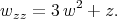
Twice integrating Eq.(3.14) with respect to we have
$U - 3--U2 - p U - C η + C = 0, ηη k2 1 2$ (3.15)

where C₁ and C₂ are arbitrary constants. This equation is well known. Using the transformations for U and by formulae
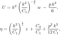$( ) 2 2 k2 -5 pk2 U = k --- w - ----, C1 6 ( 2) 15 2 2 η = -k- z + C2- + p--k--, C1 C1 12 C1$ (3.16)

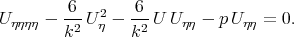
we have the first Painlevé equation [4, 7]
$wzz = 3w2 + z.$ (3.17)

The solutions of Eq. (3.17) are the Painlevé transcendents.

For the case C = 0 1 from Eq.(3.15) we obtain the equation in the form
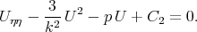$3 2 U ηη - --2 U - pU + C2 = 0. k$ (3.18)

Multiplying Eq.(3.18) on U η we have
$U 2- 2--U3 - p U2 + 2 C2U + C3 = 0, η k2$ (3.19)

where C₃ is an arbitrary constant.

The general solution of Eq. (3.19) is found via the Weierstrass elliptic function [45, 46]. We can see, that there is no need to look for the exact solutions of Eq. (3.13). This solution is expressed via the general solution of well known Eqs. (3.17) and (3.19).

Example 2c. Reduction of the Ito equation by Khani [47]
ϕxtt + ϕxxxxt + 6ϕxx ϕxt + 3ϕx ϕxxt + 3 ϕxxxϕt = 0.
(3.20)

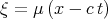
Eq. (3.20) was studied by Khani [47]. The author looked for the solutions of Eq. (3.20) taking the travelling wave into account
ϕ = ψ (ξ), ψ = k(x - λ t).
(3.21)

Substituting (3.21) into (3.20) when λ ⁄= 0 and k ⁄= 0 we obtain the equation in the form
λψ - k2ψ - 6k ψ ψ - 6 kψ ψ = 0. ξξξ ξξξξξ ξξ ξξ ξ ξξξ
(3.22)

Twice integrating Eq. (3.22) with respect to we have
λ ψξ - k2 ψξξξ - 3 k(ψ ξ)2 + C3 ξ + C4 = 0,
(3.23)
where C₃ and C₄ are arbitrary constants.

The author [47] looked for solution of Eq.(3.23) when C3 = C4 = 0 using the Exp - function method.

In fact, denoting ψ = V (ξ) ξ in Eq.(3.23) we get the following equation
k2 Vξξ + 3 kV 2 - λ V - C3 ξ - C4 = 0.
(3.24)

Eq. (3.24) is equivalent to Eq. (3.15). The solutions of this equation are expressed for C3 ⁄= 0 as the first Painlevé transcendents [4, 7] (see the previous example). For C = 0 3 the solutions of Eq. (3.24) can be obtained using the Weierstrass elliptic function. So we need not to search for the solutions of Eq. (3.22) as well.

Example 2d. Reduction of the (3+1) - dimensional Jimbo - Miva equation by Öziş and Aslan [48]
$uxxxy + 3 uy uxx + 3 uxuxy + 2 uyt - 3 uxz = 0.$ (3.25)

Using the travelling wave 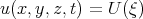u(x,y,z,t) = U (ξ) , ξ = kx + m y + r z + w t Eq. (3.25) can be written as the nonlinear ordinary differential equation
$3 2 k m Uξξξξ + 6 k m Uξ U ξξ + (2 m w - 3 kr )Uξξ = 0.$ (3.26)

The authors [48] applied the Exp - function method to Eq.(3.26) to obtain ”the exact and explicit generalized solitary solutions in more general forms”.

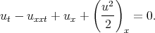
But integrating Eq.(3.26) with respect to we obtain
$3 2 2 k m U ξξξ + 3 k m U ξ + (2m w - 3 kr)U ξ = C5,$ (3.27)

where C₅ is an arbitrary constant. Denoting U ξ = V we get
$k3 m V + 3k2 m V 2 + (2m w - 3k r)V = C . ξξ 5$ (3.28)

Multiplying Eq.(3.28) on we have the equation in the form
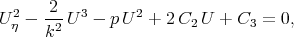
$2 2m w - 3k r 2C5 V 2ξ + --V 3 + -------3-----V 2 - ---3 V - C6 = 0, k m k mk$ (3.29)

where C₆ is an arbitrary constant. The general solution can be found using the Weierstrass elliptic function. The solution of Eq.(3.26) is found by the integral
$∫ U = V dξ.$ (3.30)

We can see that Eq.(3.27) has the general solution (3.30) and all partial cases can be found from the general solution of Eq.(3.30).

Example 2e. Reduction of the Benjamin - Bona - Mahony equation [49]
$( ) u2 ut - uxxt + ux + 2-- = 0. x$ (3.31)

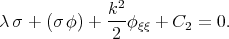
Eq. (3.31) was considered by Ganji and co - authors [49]. In terms of the travelling wave 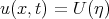u(x,t) = U (η ) , η = kx - ω t they obtained the equation
$k2 ω Uηηη + kU U η + (k - ω)U η = 0.$ (3.32)

Using the Exp - function method the authors [49] looked for the solitary wave solutions of Eq.(3.32).

Integrating Eq. (3.32) with respect to we have
$k2 ω U + 1-k U2 + (k - ω) U + C = 0. ηη 2 1$ (3.33)

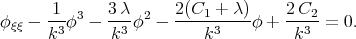
Multiplying Eq.(3.33) on U η and integrating the result with respect to again we obtain the equation
$k2 ω U 2+ k-U3 + (k - ω) U2 + 2 C1 + C2 = 0. η 3$ (3.34)

The solution of Eq.(3.34) can be given by the Weierstrass elliptic function [4, 7, 45, 46]. We can see that the authors [49] obtained the known solitary wave solutions of Eq.(3.31).

Example 2f. Reduction of the Sharma - Tasso - Olver equation by Erbas and Yusufoglu [50]
$( 3) 3- ( 2) ut + α u x + 2 α u xx + αuxxx = 0.$ (3.35)

Taking the travelling wave 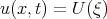u(x,t) = U (ξ ) , ξ = μ (x - c t) the authors [50] obtained the reduction of Eq.(3.35) in the form
$2 3 α μ U ξξ + 3 α μU U ξ + αU - cU = 0.$ (3.36)

The authors of [50] used the Exp - function method to find ”new solitonary solutions”, but they left out of their account that using the transformation
$Fξ- U = μ F$ (3.37)

Eq.(3.36) can be transformed to the linear equation
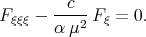$--c-- F ξξξ - α μ2 Fξ = 0.$ (3.38)

The solution of Eq.(3.38) takes the form
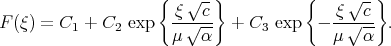${ √ -} { √ -} ξ---c- ξ---c- F (ξ) = C1 + C2 exp μ √α- + C3 exp - μ √ α- .$ (3.39)

Substituting the solution (3.39) into the transformation (3.37) we obtain the solution of Eq.(3.36) in the form
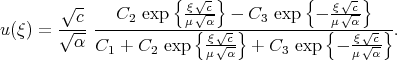$√ - { ξ√c-} { ξ√c-} c C2 exp μ√α- - C3 exp - μ√-α- u(ξ) = √-α- ------------{-ξ√c}----------{---ξ√c-}. C1 + C2 exp μ√α + C3 exp - μ√α$ (3.40)

Certainly all the solutions obtained by means of the Exp - function method can be found from solution (3.40).

Example 2g. Reduction of the dispersive long wave equations by Abdou [35]
$vt + v vx + wx = 0, 1 wt + (vw )x + --vxxx = 0. 3$ (3.41)

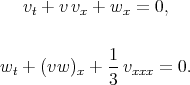
Using the wave transformations 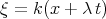w(x, t) = σ (ξ ) , v(x,t) = ϕ(ξ) , ξ = k(x + λ t) , the system of equations (3.41) can be written in the form
$λϕ ξ + ϕ ϕξ + σξ = 0,$ (3.42)

$k2- λσ ξ + (σ ϕ)ξ + 2 ϕ ξξξ = 0.$ (3.43)

Abdou [35] looked for solutions of the system of equations (3.42) and (3.43) taking ”the extended tanh method” into account.

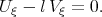
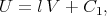
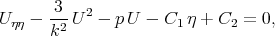
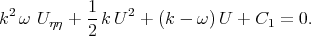
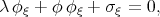
Integrating Eqs. (3.42) and (3.43) with respect to we obtain
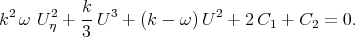
$1- 2 σ = - C1 - λ ϕ - 2 ϕ ,$ (3.44)

$2 λ σ + (σ ϕ) + k-ϕ ξξ + C2 = 0. 2$ (3.45)

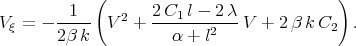
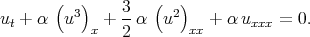
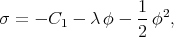
Substituting the value of from (3.44) into Eq.(3.45) we have
$-1- 3 3λ- 2 2(C1-+--λ) 2-C2- ϕ ξξ - k3 ϕ - k3 ϕ - k3 ϕ + k3 = 0.$ (3.46)

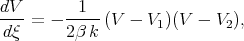
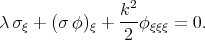
Multiplying Eq.(3.46) on ϕ ξ and integrating the equation with respect to , we have the equation in the form
$1 3λ (C + λ ) 2 C ϕ2ξ - ----ϕ4 - ---ϕ3 - ---1-----ϕ2 + ---2-ϕ + C3 = 0. 2k3 k3 k3 k3$ (3.47)

The general solution of Eq.(3.47) is determined via the Jacobi elliptic function [7]. The variable is found by the formula (3.44) and there is no need to look for the exact solutions of the Eqs.(3.42) and (3.43).

Unfortunately we have many similar examples. Some of them are also presented in our recent work [46].

The EqWorld website presents extensive information on solutions to various classes of ordinary differential equations, partial differential equations, integral equations, functional equations, and other mathematical equations.

Seven common errors in finding exact solutions of nonlinear differential equations © N.A. Kudryashov Communications in Nonlinear Science and Numerical Simulation (to be pubslished in 2009)

Contents

3. Second error: some authors do not use the known general solutions of ordinary differential equations

Seven common errors in finding exact solutions of nonlinear differential equations
© N.A. Kudryashov
Communications in Nonlinear Science and Numerical Simulation (to be pubslished in 2009)